library(tidyverse)
library(jsonlite)
library(janitor)
theme_set(theme_minimal())2 Aggregating and linking trace data
Individual digital trace data offer a rich source of information about user activities, preferences, and behaviors. To gain comprehensive insights, it is frequently necessary to aggregate the data for multiple users, and combine these datasets with other relevant information.
We begin by loading the necessary packages and set a minimal visual theme for our plots using theme_minimal().
2.1 Aggregating trace data
2.1.1 Creating sessions
A common task when using digital trace data is creating usage sessions, based on some criterium. Here we use the Instagram DDP again, which we load from the JSON file.
insta_views <- jsonlite::fromJSON("data/posts_viewed.json", simplifyVector = FALSE) |>
  map(unlist) |> # all fields as a flat list
  map_dfr(~ tibble(
    timestamp = .x[[1]],
    url = .x[[4]],
    account = .x[[length(.x) - 3]],
  )) |>
  mutate(
    timestamp = as.POSIXct(as.numeric(timestamp), origin = "1970-01-01"),
  ) |>
  arrange(timestamp)

insta_views
# A tibble: 254 × 3
timestamp url account
<dttm> <chr> <chr>
1 2026-04-13 15:58:57 https://www.instagram.com/p/DW8jWyqjTuT/ funk
2 2026-04-13 16:00:07 https://www.instagram.com/p/DXEaAIkCJAo/ tagesschau
3 2026-04-13 16:01:47 https://www.instagram.com/p/DXB3hOPmuxL/ zeit
4 2026-04-13 16:01:47 https://www.instagram.com/p/DXEDda4ls6E/ spiegelmagazin
5 2026-04-13 16:02:28 https://www.instagram.com/p/DXCgqkjCBHL/ szmagazin
# ℹ 249 more rowsNext, we aim to identify browsing sessions based on the time elapsed between consecutive post views. We calculate the time difference since the last viewed post and define a new session if this duration exceeds one hour (3600 seconds) or if it’s the first view. We then create a session_id by cumulatively counting these new session starts.
insta_views <- insta_views |>
  mutate(
    since_last_post = as.numeric(timestamp - lag(timestamp)),
    new_session = as.numeric(since_last_post) > 3600 | is.na(since_last_post),
    session_id = cumsum(new_session)
  )

insta_views
# A tibble: 254 × 6
timestamp url account since_last_post new_session session_id
<dttm> <chr> <chr> <dbl> <lgl> <int>
1 2026-04-13 15:58:57 https://ww… funk NA TRUE 1
2 2026-04-13 16:00:07 https://ww… tagess… 70 FALSE 1
3 2026-04-13 16:01:47 https://ww… zeit 100 FALSE 1
4 2026-04-13 16:01:47 https://ww… spiege… 0 FALSE 1
5 2026-04-13 16:02:28 https://ww… szmaga… 41 FALSE 1
# ℹ 249 more rowsFinally, to understand the distribution of session lengths, we count the number of post views within each identified session.
insta_views |>
  count(session_id)
# A tibble: 18 × 2
session_id n
<int> <int>
1 1 56
2 2 20
3 3 1
4 4 19
5 5 7
# ℹ 13 more rows2.1.2 Combining multiple data sets
Another frequent task is to combine multiple donated or collected data files, one by each study participant. We begin by listing and reading all relevant data files within the specified directory. The subsequent code snippet employs the list.files() function to generate list of all JSON files within the data/tt_ddp/ directory.
json_files <- list.files("data/tt_ddp/", pattern = "*.json", full.names = TRUE)
json_files
[1] "data/tt_ddp//1.json" "data/tt_ddp//2.json" "data/tt_ddp//3.json"
[4] "data/tt_ddp//4.json"The following code performs a series of transformations to read and combine the TikTok viewing history from multiple respondents. Initially, map(jsonlite::fromJSON) parses each JSON file into a list. Subsequently, map(~ .x$Activity$Video Browsing History$VideoList) extracts the video browsing history data frame from each parsed list. Finally, bind_rows() combines these data frames into a single tibble while adding a respondent_id column to maintain the original id of each data set. We add the usual time and date columns and clean up the variable names.
df_combined <- json_files |>
  map(jsonlite::fromJSON) |>
  map(~ .x$Activity$`Video Browsing History`$VideoList) |>
  bind_rows(.id = "respondent_id") |>
  as_tibble() |>
  mutate(
    day = as.Date(Date),
    hour = lubridate::hour(Date),
    weekday = lubridate::wday(Date, label = TRUE, week_start = 1)
  ) |>
  janitor::clean_names()

df_combined
# A tibble: 12 × 7
respondent_id date title url day hour weekday
<chr> <chr> <chr> <chr> <date> <int> <ord>
1 1 2024-01-15 10:05:00 Example Vide… http… 2024-01-15 10 Mon
2 1 2024-01-15 12:35:00 Example Vide… http… 2024-01-15 12 Mon
3 1 2024-01-16 14:05:00 Example Vide… http… 2024-01-16 14 Tue
4 2 2024-02-01 08:05:00 Funny Cats C… http… 2024-02-01 8 Thu
5 2 2024-02-01 11:35:00 Amazing Danc… http… 2024-02-01 11 Thu
# ℹ 7 more rowsThe result is a long data file with an ID variable for each user, which we can then process and analyze. The same procedure works for most files, and we only need to adapt the map() calls for different file types or different fields to access.
2.2 Linking digital trace data
For many research questions, it is helpful or even necessary to link digital trace data with other data, e.g. survey responses from the participants, or content data from the consumed posts, videos or music tracks. In this example, we will use a subset of an experience sampling study, where respondents answered questions about their Spotify use, but also donated their listening histories.
We begin by reading the spotify_history.tsv file into an R data frame. This initial step allows us to inspect the structure and content of the raw digital trace data we will be working with.
spotify_history <- read_tsv("data/spotify_history.tsv")
spotify_history
# A tibble: 2,325 × 5
participant_id tstamp track_id context_type context_id
<chr> <dttm> <chr> <chr> <chr>
1 127XY52RUE 2023-02-02 09:59:06 6HSXNV0b4M4cLJ7ljg… <NA> <NA>
2 127XY52RUE 2023-02-02 12:59:25 5IHk3ooYCKJGYk7qCU… playlist 37i9dQZF1…
3 127XY52RUE 2023-02-03 15:01:23 5IHk3ooYCKJGYk7qCU… playlist 37i9dQZF1…
4 127XY52RUE 2023-02-03 15:03:41 1dWUBCoztAMZcqec1C… album 3399XMtHg…
5 127XY52RUE 2023-02-03 15:04:40 3vLByi1CdmNJPpTtOd… album 3399XMtHg…
# ℹ 2,320 more rowsNext, we want to count the number of participants and the number of listening events recorded for each participant in our dataset.
spotify_history |>
  count(participant_id, sort = TRUE)
# A tibble: 20 × 2
participant_id n
<chr> <int>
1 7VC5977MW1 176
2 QMH2H4NAKS 169
3 FFP6XWSS99 159
4 Z2L134QXCR 150
5 UQ39DMWF4F 147
# ℹ 15 more rowsTo explore the temporal dynamics of our data, we will now calculate the number of unique active users and the total number of songs listened to on each day. This involves extracting the date from the timestamp, grouping the data by day, and then summarizing the distinct participant IDs and the total number of tracks listened to.
user_counts <- spotify_history |>
  mutate(day = as.Date(tstamp)) |>
  group_by(day) |>
  summarise(
    n_users = n_distinct(participant_id),
    n_songs = n()
  )

user_counts
# A tibble: 44 × 3
day n_users n_songs
<date> <int> <int>
1 2023-02-02 1 2
2 2023-02-03 1 18
3 2023-02-06 2 11
4 2023-02-07 1 1
5 2023-02-08 1 2
# ℹ 39 more rowsWe can visualize this using a bar plot showing the number of active users for each day in our observation period.
user_counts |>
  ggplot(aes(x = day, y = n_users)) +
  geom_col() +
  labs(title = "Active users per day", x = "Day", y = "Active users")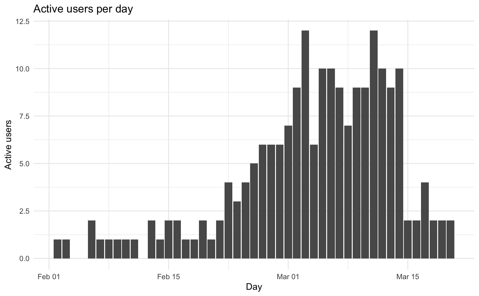
2.2.1 Adding survey data
Now, we introduce the cross-sectional survey data containing demographic information and music preferences about our participants. This dataset will allow us to link listening behavior with user characteristics.
spotify_respondents <- read_tsv("data/spotify_respondents.tsv")
spotify_respondents
# A tibble: 31 × 28
participant_id age gender frq_album frq_faves frq_ownplaylist
<chr> <dbl> <dbl> <dbl> <dbl> <dbl>
1 LQLLLF255U 20 2 2 5 3
2 2GH1CK19LH 20 2 3 4 5
3 CXEBG98UPG 18 2 2 5 5
4 CEGPUS95SC 18 2 5 2 5
5 SWC8Y6A2AT 27 2 4 1 4
# ℹ 26 more rows
# ℹ 22 more variables: frq_userplaylist <dbl>, frq_radio <dbl>,
# frq_edplaylist <dbl>, frq_charts <dbl>, frq_other <dbl>,
# genresr_residual <dbl>, genresr_pop <dbl>, genresr_rock <dbl>,
# genresr_religious <dbl>, genresr_reggae <dbl>, genresr_jazz <dbl>,
# genresr_rap <dbl>, genresr_dance <dbl>, genresr_indie <dbl>,
# genresr_metal <dbl>, genresr_klassik <dbl>, genresr_punk <dbl>, …To connect the digital trace data with the survey responses, we perform a so-called left join operation. This merges the spotify_history data frame with spotify_respondents based on the common participant_id, allowing us to analyze listening patterns in relation to demographics. Left join means that all rows on the left-hand side are kept, even if there are no matching cases on the right-hand side.
spotify_history |>
  left_join(spotify_respondents, by = "participant_id")
# A tibble: 2,325 × 32
participant_id tstamp track_id context_type context_id age
<chr> <dttm> <chr> <chr> <chr> <dbl>
1 127XY52RUE 2023-02-02 09:59:06 6HSXNV0b4M4c… <NA> <NA> 21
2 127XY52RUE 2023-02-02 12:59:25 5IHk3ooYCKJG… playlist 37i9dQZF1… 21
3 127XY52RUE 2023-02-03 15:01:23 5IHk3ooYCKJG… playlist 37i9dQZF1… 21
4 127XY52RUE 2023-02-03 15:03:41 1dWUBCoztAMZ… album 3399XMtHg… 21
5 127XY52RUE 2023-02-03 15:04:40 3vLByi1CdmNJ… album 3399XMtHg… 21
# ℹ 2,320 more rows
# ℹ 26 more variables: gender <dbl>, frq_album <dbl>, frq_faves <dbl>,
# frq_ownplaylist <dbl>, frq_userplaylist <dbl>, frq_radio <dbl>,
# frq_edplaylist <dbl>, frq_charts <dbl>, frq_other <dbl>,
# genresr_residual <dbl>, genresr_pop <dbl>, genresr_rock <dbl>,
# genresr_religious <dbl>, genresr_reggae <dbl>, genresr_jazz <dbl>,
# genresr_rap <dbl>, genresr_dance <dbl>, genresr_indie <dbl>, …Let’s calculate the total number of tracks listened to by each participant. This aggregation provides a summary measure of individual listening activity, which we can link back to the survey data.
spotify_counts <- spotify_history |>
  count(participant_id, name = "n_tracks")

spotify_counts
# A tibble: 20 × 2
participant_id n_tracks
<chr> <int>
1 127XY52RUE 106
2 2GH1CK19LH 103
3 4CFCAYX932 136
4 6SVQ1NXTKH 135
5 7VC5977MW1 176
# ℹ 15 more rowsWe add the calculated number of tracks listened to by each participant to the survey data by performing a left join between spotify_respondents and spotify_counts using participant_id and then select a subset of relevant variables for further analysis.
spotify_respondents |>
  left_join(spotify_counts, by = "participant_id") |>
  select(participant_id, age, gender, n_tracks)
# A tibble: 31 × 4
participant_id age gender n_tracks
<chr> <dbl> <dbl> <int>
1 LQLLLF255U 20 2 123
2 2GH1CK19LH 20 2 103
3 CXEBG98UPG 18 2 58
4 CEGPUS95SC 18 2 NA
5 SWC8Y6A2AT 27 2 110
# ℹ 26 more rowsNotably, there are a few cases with missing track count information, since we left-joined to the survey data with a larger number of participants. If we wanted to keep only complete information, we could use the right_join() or inner_join() functions.
2.2.2 Adding song data
The spotify_songs.tsv dataset contains various audio features for each track, identified by the id column.
spotify_songs <- read_tsv("data/spotify_songs.tsv")
spotify_songs
# A tibble: 1,596 × 21
id release_date duration_ms popularity artist_id danceability energy key
<chr> <chr> <dbl> <dbl> <chr> <dbl> <dbl> <dbl>
1 2PFnw… 2020-07-17 125051 61 6TLwD7HP… NA NA NA
2 5nWgD… 2019-08-16 146826 58 1U0pXcl8… NA NA NA
3 46sBh… 2021-08-18 132580 63 1KS3HFd7… NA NA NA
4 5WFsl… 2020-09-18 170785 42 1ul8iLt2… NA NA NA
5 43vdI… 2013-04-05 227057 18 2CTeIzSe… 0.629 0.289 6
# ℹ 1,591 more rows
# ℹ 13 more variables: loudness <dbl>, mode <dbl>, speechiness <dbl>,
# acousticness <dbl>, instrumentalness <dbl>, liveness <dbl>, valence <dbl>,
# tempo <dbl>, type <chr>, uri <chr>, track_href <chr>, analysis_url <chr>,
# time_signature <dbl>We now create a complete dataset by merging the listening history, survey responses, and song features. We perform sequential left join operations, first joining spotify_history with spotify_respondents by participant_id, and then joining the result with spotify_songs using the track_id. Note that the track id is called id in the song data. We could either rename the column, or specify the respective names in the by argument of the join function.
spotify_complete <- spotify_history |>
  left_join(spotify_respondents, by = "participant_id") |>
  left_join(spotify_songs, by = c("track_id" = "id"))
spotify_complete
# A tibble: 2,325 × 52
participant_id tstamp track_id context_type context_id age
<chr> <dttm> <chr> <chr> <chr> <dbl>
1 127XY52RUE 2023-02-02 09:59:06 6HSXNV0b4M4c… <NA> <NA> 21
2 127XY52RUE 2023-02-02 12:59:25 5IHk3ooYCKJG… playlist 37i9dQZF1… 21
3 127XY52RUE 2023-02-03 15:01:23 5IHk3ooYCKJG… playlist 37i9dQZF1… 21
4 127XY52RUE 2023-02-03 15:03:41 1dWUBCoztAMZ… album 3399XMtHg… 21
5 127XY52RUE 2023-02-03 15:04:40 3vLByi1CdmNJ… album 3399XMtHg… 21
# ℹ 2,320 more rows
# ℹ 46 more variables: gender <dbl>, frq_album <dbl>, frq_faves <dbl>,
# frq_ownplaylist <dbl>, frq_userplaylist <dbl>, frq_radio <dbl>,
# frq_edplaylist <dbl>, frq_charts <dbl>, frq_other <dbl>,
# genresr_residual <dbl>, genresr_pop <dbl>, genresr_rock <dbl>,
# genresr_religious <dbl>, genresr_reggae <dbl>, genresr_jazz <dbl>,
# genresr_rap <dbl>, genresr_dance <dbl>, genresr_indie <dbl>, …Finally, we want to explore whether there are differences in the average danceability of the music listened to by male and female respondents across different days of the week. We first prepare the data by extracting the day of the week, recoding the gender variable, and then grouping by gender and day. We then calculate the mean danceability and visualize the results using a line plot with points.
spotify_complete |>
  mutate(
    wday = lubridate::wday(tstamp, label = TRUE, week_start = 1),
    gender = if_else(gender == 1, "male", "female")
  ) |>
  group_by(gender, wday) |>
  summarise(dance = mean(danceability, na.rm = TRUE)) |>
  ggplot(aes(
    x = wday, y = dance,
    color = gender, group = gender
  )) +
  geom_line() +
  geom_point() +
  labs(x = "Day of the week", y = "Average danceability", color = "Respondent gender")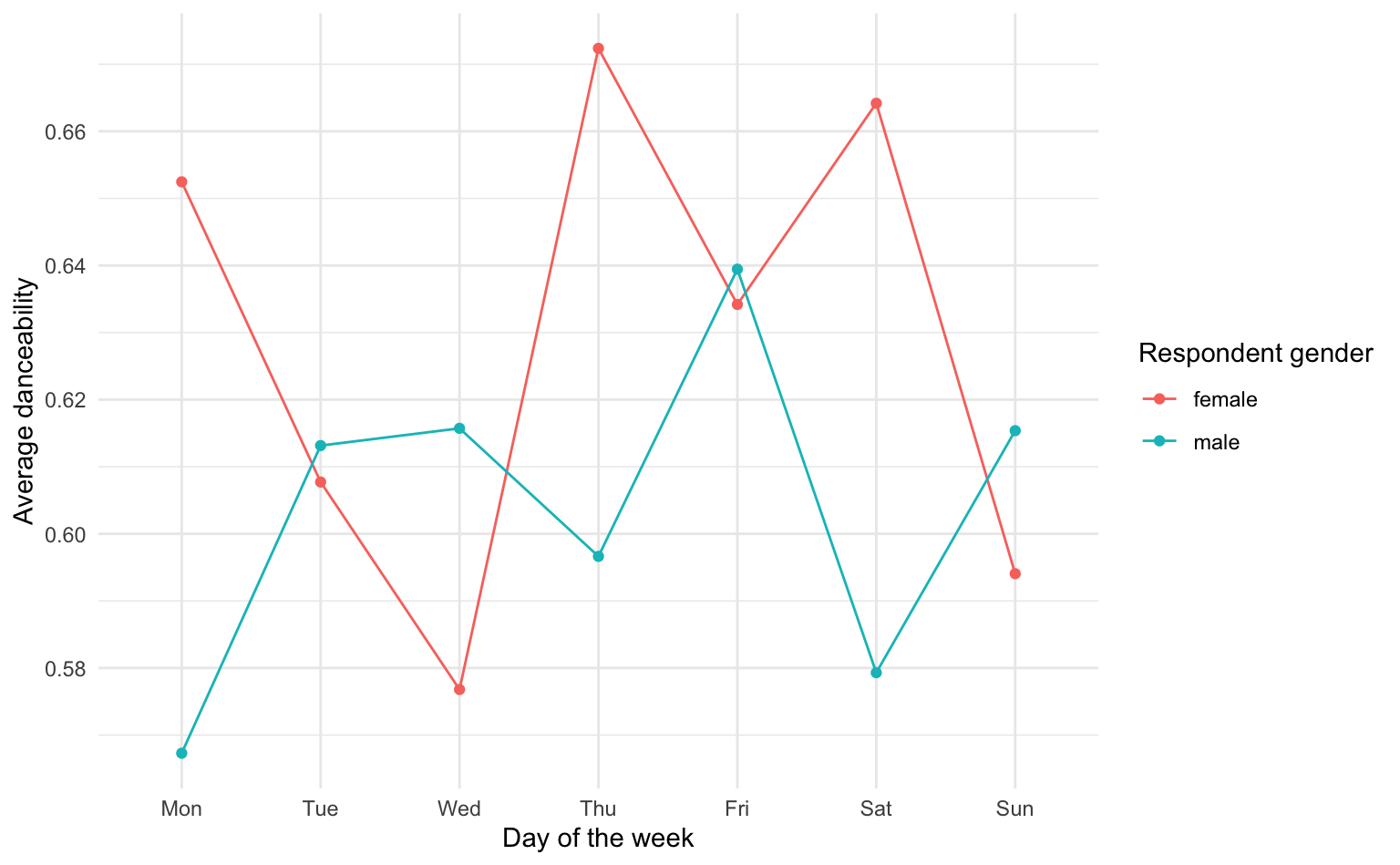
Male respondents listen to less danceable music, and Thursdays and Saturdays are for dancing (for female respondents at least)!
2.3 Homework
- Create a session variable for the Spotify listing data. Keep in mind that the data contains logs from multiple users, so you need to group the data frame per user before creating the session variable. How long is the average Spotify listening session?
- Use the Spotify data for any interesting analysis you can think of. Visualize the results.
- Bonus: Download your own Spotify DDP data or a publicly available dataset and try to read and analyze the data.