library(tidyverse)
library(ndjson)
library(janitor)
library(emoji)
library(taylor)
library(ellmer)
theme_set(theme_minimal())4 Automatic text analysis
We begin by loading the necessary packages and set a minimal visual theme for our plots using theme_minimal(). Specifically, we use ndjson for working with NDJSON files, janitor for data cleaning, emoji for handling emojis, taylor for data, and finally ellmer for interacting with different LLM APIs.
4.1 Working with text data
To get started, we’re importing our Zeeschuimer TikTok data, which is in a ndjson format. Then, we’ll clean up the column names and select the relevant ones.
tt_data <- ndjson::stream_in("data/zeeschuimer-export-tiktok.ndjson") |>
  bind_rows() |>
  as_tibble() |>
  set_names(str_remove_all, pattern = "^data.") |>
  janitor::clean_names() |>
  select(video_id, author = author_unique_id, desc)

tt_data
# A tibble: 70 × 3
video_id author desc
<chr> <chr> <chr>
1 7437889533078801696 mr.eingeschraenkt "Läuft immer so ab"
2 7431952376220618017 fakteninsider "Das passiert wenn du ein porenpflaster…
3 7422341529571724577 besttrendvideos "Da war Candy Crush level 6589 wieder w…
4 7427553745447292193 pubity "Oddly satisfying flooring 😍 @Jaycurlss…
5 7407090202813943072 martin._.yk "😮💨#foryoupage #real #school #trendingvi…
# ℹ 65 more rowsIn the next step, we’ll try out some basic string manipulation: converting the description desc text to title case and all lowercase.
tt_data |>
  mutate(
    desc_title = stringr::str_to_title(desc),
    desc_lower = stringr::str_to_lower(desc)
  ) |>
  select(video_id, desc_title, desc_lower)
# A tibble: 70 × 3
video_id desc_title desc_lower
<chr> <chr> <chr>
1 7437889533078801696 "Läuft Immer So Ab" "läuft im…
2 7431952376220618017 "Das Passiert Wenn Du Ein Porenpflaster Benutz… "das pass…
3 7422341529571724577 "Da War Candy Crush Level 6589 Wieder Wichtige… "da war c…
4 7427553745447292193 "Oddly Satisfying Flooring 😍 @Jaycurlsstudios … "oddly sa…
5 7407090202813943072 "😮💨#Foryoupage #Real #School #Trendingvideo " "😮💨#foryou…
# ℹ 65 more rows4.2 Counting words and other things
4.2.1 Counting content using regular expressions
Next, we move to some actual content analysis, albeit a very simplistic one: we are calculating various characteristics of our text, such as the number of characters, words, hashtags, emojis, and occurrences of a specific word (“love”), all using regular expressions. Regular expressions are patterns used to match character combinations in strings.
We use multiple patterns:
\\w+: This matches one or more “word characters” (letters, numbers, and underscores).#\\w+: This looks for a hashtag symbol (#) followed by one or more word characters, which helps us identify hashtags.\\blove\\b: The\\bis a special marker for a “word boundary.” This ensures we only count the whole word “love” and not parts of other words like “lovely” or “glove.”
tt_data |>
  mutate(
    n_chars = stringr::str_length(desc),
    n_words = stringr::str_count(desc, "\\w+"),
    n_hashtags = stringr::str_count(desc, "#\\w+"),
    n_emojis = emoji::emoji_count(desc),
    n_love = stringr::str_count(desc, "\\blove\\b")
  ) |>
  select(video_id, n_chars, n_words, n_hashtags, n_emojis, n_love)
# A tibble: 70 × 6
video_id n_chars n_words n_hashtags n_emojis n_love
<chr> <int> <int> <int> <int> <int>
1 7437889533078801696 17 4 0 0 0
2 7431952376220618017 123 15 8 1 0
3 7422341529571724577 134 18 5 2 0
4 7427553745447292193 115 10 5 1 0
5 7407090202813943072 44 5 4 2 0
# ℹ 65 more rows4.2.2 Extracting content using regular expressions
Next, we extract all hashtags from the descriptions using the #\\w+ regular expression we just discussed and then count their occurrences to find the most frequent ones.
tt_data |>
  mutate(hashtags = stringr::str_extract_all(desc, "#\\w+")) |>
  unnest(hashtags) |>
  count(hashtags, sort = TRUE)
# A tibble: 234 × 2
hashtags n
<chr> <int>
1 #fyp 18
2 #fy 11
3 #foryou 7
4 #viral 6
5 #foryoupage 4
# ℹ 229 more rowsSimilarly, we’ll extract and count the emojis to see which ones are used most often.
tt_data |>
  mutate(emojis = emoji::emoji_extract_all(desc)) |>
  unnest(emojis) |>
  count(emojis, sort = TRUE)
# A tibble: 45 × 2
emojis n
<chr> <int>
1 😭 9
2 ✨ 8
3 🥰 5
4 😂 4
5 😇 3
# ℹ 40 more rows4.3 Dictionary coding
Dictionary coding, i.e. classifying text according to the words contained in it, is one of the oldest approaches in automatic content analysis. There are multiple R packages that specialize in dictionary coding, but we’ll just use regular expressions for a quick and dirty solution.
First, we’re loading the Taylor Swift lyrics data, which will serve as our example for dictionary coding,
taylor_lyrics <- taylor::taylor_all_songs |>
  unnest(lyrics) |>
  select(album_name, album_release, track_name, lyric)

taylor_lyrics
# A tibble: 18,172 × 4
album_name album_release track_name lyric
<chr> <date> <chr> <chr>
1 Taylor Swift 2006-10-24 Tim McGraw "He said the way my blue eyes shined"
2 Taylor Swift 2006-10-24 Tim McGraw "Put those Georgia stars to shame that …
3 Taylor Swift 2006-10-24 Tim McGraw "I said, \"That's a lie\""
4 Taylor Swift 2006-10-24 Tim McGraw "Just a boy in a Chevy truck"
5 Taylor Swift 2006-10-24 Tim McGraw "That had a tendency of gettin' stuck"
# ℹ 18,167 more rowsNow, we’ll define regular expressions for “me,” “you,” and “others” and then use them to detect the presence of these pronouns in each lyric. Notice again the use of \\b for word boundaries to ensure we match only the full words. For example, \\b(me|myself|i|my|mine)\\b looks for “me”, “myself”, “i”, “my”, or “mine” as whole words ((a|b) means a OR b). We then summarize the proportion of mentions per album.
me <- "\\b(me|myself|i|my|mine)\\b"
you <- "\\b(you|your|yours)\\b"
others <- "\\b(they|them|their|he|him|his|she|her)\\b"

taylor_results <- taylor_lyrics |>
  mutate(lyric = str_to_lower(lyric)) |>
  mutate(
    me = str_detect(lyric, me),
    you = str_detect(lyric, you),
    others = str_detect(lyric, others)
  ) |>
  group_by(album_name, album_release) |>
  summarise_if(is.logical, mean)

taylor_results
# A tibble: 18 × 5
# Groups: album_name [18]
album_name album_release me you others
<chr> <date> <dbl> <dbl> <dbl>
1 1989 2014-10-27 0.326 0.338 0.0668
2 1989 (Taylor's Version) 2023-10-27 0.378 0.386 0.0751
3 Beautiful Eyes 2008-07-15 0.677 0.478 0.108
4 Fearless 2008-11-11 0.554 0.510 0.0706
5 Fearless (Taylor's Version) 2021-04-09 0.530 0.479 0.0590
# ℹ 13 more rowsFinally, we’ll visualize the trend of personal pronoun usage across Taylor Swift’s albums over time.
taylor_results |>
  gather(category, value, me:others) |>
  ggplot(aes(x = album_release, y = value, color = category)) +
  geom_line() +
  labs(x = "Publication year", y = "Proportion of mentions per album", color = "Lyrics mention...")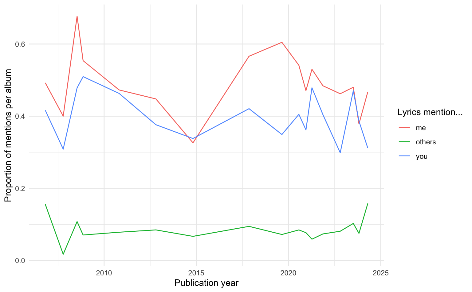
4.4 Zero-shot text classification
In the remainder of this session, we’ll use a LLM API to try out different coding tasks. We use the package ellmer which supports many commercial APIs, including Google Gemini, ChatGPT, or local models using Ollama. The JGU has recently rolled out its own JGU LLM API which follows the OpenAI messaging standard.
4.4.1 LLM API calling
Commercial APIs rely on authentication tokens, which need to be provided in any request. Since we are using the OpenAI API, we need to set the API key, which can be found in your account settings. Note that we will be using the internal JGU API, so we need our JGU-specific key.
# USE JGU API KEY, not original OPENAI KEY
JGU_API_KEY <- "XYZ"
As a first test, we request a dad joke, creating a jgu_kiobject using the chat_openai_compatible() function and its chat() method. Since we are using the JGU API, we need to set the base_url, credentials, and model parameters accordingly.
jgu_ki <- chat_openai_compatible(
  base_url = "https://ki-chat.uni-mainz.de/api",
  model = "Qwen3 235B VL",
  api_args = list(temperature = 0),
  credentials = function() {
    JGU_API_KEY
  }
)
jgu_ki$chat("Tell me a dad joke!")
Why don’t scientists trust atoms?
…because they make up everything! 😄
*(Classic dad joke — groan-worthy, but scientifically accurate!)*Great, our API calls to the JGU KI model work.
4.4.2 A basic coding function
In order to make our automatic coding easier, we can define a task and types, and use ellmer::interpolate() to create the prompts, and parallel_chat_structured() to run them in parallel.
example_df <- tt_data |>
  head(5) |>
  select(video_id, desc)

my_task <- "Detect the language of the text. Provide the official ISO language code only."
my_types <- type_object(language = type_string(description = "Language code"))

tasks <- ellmer::interpolate("{{my_task}}\nText: {{example_df$desc}}")
results_lang <- parallel_chat_structured(jgu_ki, tasks, my_types)

bind_cols(example_df, results_lang)
# A tibble: 5 × 3
video_id desc language
<chr> <chr> <chr>
1 7437889533078801696 "Läuft immer so ab" de
2 7431952376220618017 "Das passiert wenn du ein porenpflaster benutzt😳… de
3 7422341529571724577 "Da war Candy Crush level 6589 wieder wichtiger,… de
4 7427553745447292193 "Oddly satisfying flooring 😍 @Jaycurlsstudios @G… en
5 7407090202813943072 "😮💨#foryoupage #real #school #trendingvideo " en 4.4.3 Multiple coding tasks
We can perform multiple coding tasks simultaneously for every description by adding multiple tasks and multiple type objects. We classify text based on a random collection of categories (sorry!): humor, hair mentions, and product placements.
tasks_multi <- "Classify the text according to the following categories:

funny: On a scale from 0 (not funny) to 5 (extremely funny), how funny is the text?
hair: Does the text mention hair? true or false
product placement: Does the text mention specific brands or products? true or false
"

types_multi <- type_object(
  funny = type_number(),
  hair = type_boolean(),
  product_placement = type_boolean()
)

tasks <- ellmer::interpolate("{{tasks_multi}}\nText: {{example_df$desc}}")
results_multi <- parallel_chat_structured(jgu_ki, tasks, types_multi)

bind_cols(example_df, results_multi)
# A tibble: 5 × 5
video_id desc funny hair product_placement
<chr> <chr> <dbl> <lgl> <lgl>
1 7437889533078801696 "Läuft immer so ab" 2 FALSE FALSE
2 7431952376220618017 "Das passiert wenn du ein p… 1 FALSE FALSE
3 7422341529571724577 "Da war Candy Crush level 6… 3 FALSE TRUE
4 7427553745447292193 "Oddly satisfying flooring … 0 FALSE FALSE
5 7407090202813943072 "😮💨#foryoupage #real #school… 0 FALSE FALSE Again, the results are simply added to the original tibble.
4.4.4 Open-ended coding
Finally, we’ll demonstrate open-ended coding, where the LLM extracts a list of product brands mentioned in the text. For this we need a list called type_array, and need to define the type of the individual items in this list. We do this for the last 5 entries in the TikTok data.
task_open <- "List all the product brands explicitly mentioned in the text."
types_open <- type_object(brands = type_array(items = type_string()))

example_df_open <- tt_data |>
  tail(5) |>
  select(video_id, desc)

tasks <- ellmer::interpolate("{{task_open}}\nText: {{example_df_open$desc}}")
results <- parallel_chat_structured(jgu_ki, tasks, types_open)

bind_cols(example_df_open, results) |>
  select(-desc) |>
  unnest(brands)
# A tibble: 5 × 2
video_id brands
<chr> <chr>
1 7434230526854073632 YSL Beauty
2 7434230526854073632 Lancôme
3 7434230526854073632 IT Cosmetics
4 7434230526854073632 Armani Beauty
5 7434230526854073632 Douglas CosmeticsAs we can see, the LLM has quite a good definition of product brands…
4.5 Homework
- Try your own content analysis using any text data you like (including our example data from previous sessions).
- (Special Swiftie Question): Why is the line graph we produced misleading for our question, and how can we fix this?