library(tidyverse)
library(jsonlite)
library(ndjson)
library(janitor)
theme_set(theme_minimal())1 Individual digital traces
Individual digital trace data can be obtained in many different ways, for example from platforms via Data Download Packages (DDP), which respondents need to request and donate, or using a browser extension called Zeeschuimer, which collects client log files for a variety of platforms. Both approaches result in one or more JSON-formatted files which we can read and analyze in R.
We begin by loading the necessary packages and set a minimal visual theme for our plots using theme_minimal().
1.1 Data Download Packages (DDP)
1.1.1 Instagram
We first look at viewed Instagram posts. Our objective is to understand the temporal patterns of post consumption, including daily, hourly, and weekly trends. We first load the Instagram post view history from a JSON file named posts_viewed.json (currently in the ads_information/ads_and_topics subdirectory), and then have to do some horrible ad hoc data extraction to get the variables we want from the data. Unfortunately, platforms change the data format all the time, so this might not work now or in the future.
insta_views <- jsonlite::fromJSON("data/posts_viewed.json", simplifyVector = FALSE) |>
  map(unlist) |> # all fields as a flat list
  map_dfr(~ tibble(
    timestamp = .x[[1]],
    url = .x[[4]],
    account = .x[[length(.x) - 3]],
    content = .x[7]
  ))
insta_views
# A tibble: 254 × 4
timestamp url account content
<chr> <chr> <chr> <chr>
1 1776088807 https://www.instagram.com/p/DXEaAIkCJAo/ tagesschau "Die schwa…
2 1776088907 https://www.instagram.com/p/DXB3hOPmuxL/ zeit "🫂 Söhne z…
3 1776088907 https://www.instagram.com/p/DXEDda4ls6E/ spiegelmagazin "Die Bunde…
4 1776088952 https://www.instagram.com/p/DWik6szkfMX/ spiegelmagazin "Collien F…
5 1776088952 https://www.instagram.com/p/DW_1aHtjhQY/ emilypfender "Are these…
# ℹ 249 more rowsTo facilitate temporal analysis, we create several new variables. We rename the account and timestamp columns for clarity. Then, we convert the UNIX timestamp to a POSIXct object, enabling us to extract the date, hour, and day of the week using functions from the base R and lubridate package, which is part of the tidyverse.
insta_views <- insta_views |>
  mutate(
    timestamp = as.POSIXct(as.numeric(timestamp), origin = "1970-01-01"),
    day = as.Date(timestamp),
    hour = lubridate::hour(timestamp),
    weekday = lubridate::wday(timestamp, label = TRUE, week_start = 1)
  )
insta_views
# A tibble: 254 × 7
timestamp url account content day hour weekday
<dttm> <chr> <chr> <chr> <date> <int> <ord>
1 2026-04-13 16:00:07 https://www.inst… tagess… "Die s… 2026-04-13 16 Mon
2 2026-04-13 16:01:47 https://www.inst… zeit "🫂 Söh… 2026-04-13 16 Mon
3 2026-04-13 16:01:47 https://www.inst… spiege… "Die B… 2026-04-13 16 Mon
4 2026-04-13 16:02:32 https://www.inst… spiege… "Colli… 2026-04-13 16 Mon
5 2026-04-13 16:02:32 https://www.inst… emilyp… "Are t… 2026-04-13 16 Mon
# ℹ 249 more rowsAs a first step, we can simply count the posts viewed by Instagram account.
insta_views |>
  count(account, sort = TRUE) |>
  head(5)
# A tibble: 5 × 2
account n
<chr> <int>
1 spiegelmagazin 55
2 zeit 31
3 zdfinfo 23
4 szmagazin 21
5 sz 20To visualize the daily trend of Instagram post views, we first count the number of views for each day. Subsequently, we use ggplot2 to create a bar chart, with the day on the x-axis and the count of views on the y-axis.
insta_views |>
  count(day) |>
  ggplot(aes(x = day, y = n)) +
  geom_col() +
  labs(title = "Instagram posts viewed per day")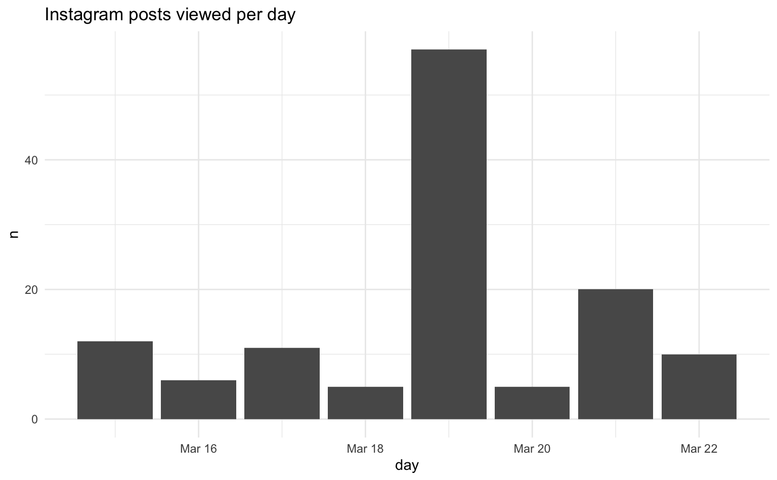
We could repeat this analysis for different time units such as the time of day (hour) or day of the week.
1.1.2 TikTok
We load the TikTok user data from a JSON file user_data.json. The JSON contains multiple fields which contain interesting data.
tiktok <- jsonlite::fromJSON("data/user_data.json")
names(tiktok)
[1] "Comment" "Direct Message" "Income+ Wallet"
[4] "Likes and Favorites" "Location Review" "Post"
[7] "Profile And Settings" "TikTok Live" "TikTok Shop"
[10] "Your Activity" Here, we analyze the history of TikTok logins to identify patterns in access frequency over time. We extract the login history from the loaded TikTok data and convert it into a tibble for easier manipulation and analysis. We then create new temporal variables – day, hour, and weekday – from the Date column, which is a parsable string. This allows us to analyze login frequency across different time scales.
tt_logins <- tiktok$`Your Activity`$`Login History`$LoginHistoryList |>
  as_tibble() |>
  mutate(
    day = as.Date(Date),
    hour = lubridate::hour(Date),
    weekday = lubridate::wday(Date, label = TRUE, week_start = 1)
  )

tt_logins
# A tibble: 12 × 9
Date IP DeviceModel DeviceSystem NetworkType Carrier day hour
<chr> <chr> <chr> <chr> <chr> <chr> <date> <int>
1 2026-04-1… 134.… iPhone13,4 iOS 26.3.1 Wi-Fi "" 2026-04-15 12
2 2026-04-1… 77.2… iPhone13,4 iOS 26.3.1 Wi-Fi "" 2026-04-15 22
3 2026-04-1… 77.2… iPhone13,4 iOS 26.3.1 Wi-Fi "" 2026-04-15 22
4 2026-04-1… 77.2… iPhone13,4 iOS 26.3.1 Wi-Fi "" 2026-04-15 22
5 2026-04-1… 176.… iPhone13,4 iOS 26.3.1 5g "" 2026-04-16 7
# ℹ 7 more rows
# ℹ 1 more variable: weekday <ord>We can then visualize the frequency of TikTok logins by counting the number of logins per day of the week.
tt_logins |>
  count(weekday) |>
  ggplot(aes(x = weekday, y = n)) +
  geom_col() +
  labs(title = "TikTok logins per day of the week")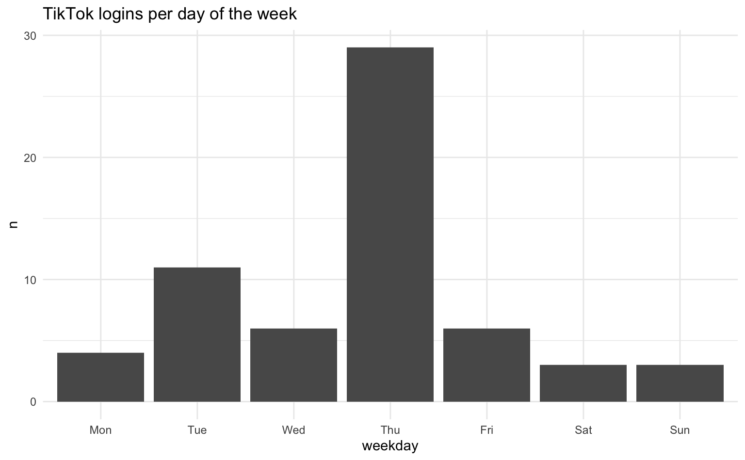
In the next step, we investigate the history of viewed TikTok videos to understand the patterns of content consumption over time. The procedure is the same as above, including converting the timestamps to multiple variables.
tt_views <- tiktok$`Your Activity`$`Watch History`$VideoList |>
  as_tibble() |>
  mutate(
    day = as.Date(Date),
    hour = lubridate::hour(Date),
    weekday = lubridate::wday(Date, label = TRUE, week_start = 1)
  )

tt_views
# A tibble: 160 × 5
Date Link day hour weekday
<chr> <chr> <date> <int> <ord>
1 2026-04-15 12:39:05 https://www.tiktokv.com/share/vi… 2026-04-15 12 Wed
2 2026-04-15 12:39:14 https://www.tiktokv.com/share/vi… 2026-04-15 12 Wed
3 2026-04-15 12:39:15 https://www.tiktokv.com/share/vi… 2026-04-15 12 Wed
4 2026-04-15 12:41:50 https://www.tiktokv.com/share/vi… 2026-04-15 12 Wed
5 2026-04-15 12:41:51 https://www.tiktokv.com/share/vi… 2026-04-15 12 Wed
# ℹ 155 more rowsNote that the data include only the viewed video URL, but no additional meta data. We would need to collect and link these data in a separate step. For now, we aggregate the viewing history data by counting the number of videos viewed on each day of the history file and display the results as a bar chart.
tt_views |>
  count(day) |>
  ggplot(aes(x = day, y = n)) +
  geom_col() +
  labs(title = "TikTok videos watched per day")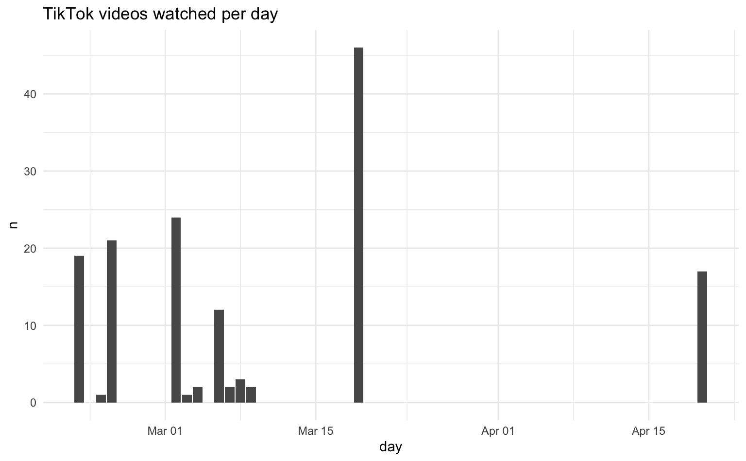
Finally, we examine the history of direct messages on TikTok to understand communication patterns, focusing on the frequency of messages with different users. We load the direct message history from the TikTok data. Since the chat history might be structured as a list of data frames, we use bind_rows() to combine them into a single tibble.
tt_dm <- tiktok$`Direct Message`$`Direct Messages`$ChatHistory |>
  bind_rows() |>
  as_tibble()

tt_dm
# A tibble: 3 × 3
Date From Content
<chr> <chr> <chr>
1 2026-04-15 12:41:33 user4912600155075 Hier ist ein Test zurück
2 2026-04-15 12:40:51 alicia.ernst 🥳🥳🥳
3 2026-04-15 12:40:42 alicia.ernst Hi das ist ein Test To understand communication frequency with different users, we count the number of messages sent by each user (identified by the From variable) and display the results in descending order of frequency.
tt_dm |>
  count(From, sort = TRUE)
# A tibble: 2 × 2
From n
<chr> <int>
1 alicia.ernst 2
2 user4912600155075 11.2 Zeeschuimer browser logs
1.2.1 Instagram
Sometimes, it is preferable to collect “live” browsing data, e.g. in a lab experiment. We collect and extract them using Zeeschuimer. Start monitoring the browser session, and export the data as an NDJSON-File afterwards. This is also one of the few ways to collect additional meta data from Instagram, so you might open a number of Instagram URLs in your browser, then Zeeschuimer will collect their data.
We begin by using the stream_in() function from the ndjson package to efficiently read the potentially large NDJSON file named zeeschuimer-export-instagram.ndjson. The streamed data, which might consist of multiple JSON objects, is then combined into a single data frame using bind_rows() and subsequently converted into a tibble. To ensure consistent and clean column names, we first remove the prefix “data.” using set_names(). Following this, we apply the clean_names() function from the janitor package to standardize the column names, typically converting them to snake_case. Next, we perform data type conversions: the taken_at column is converted to POSIXct format, and the seen_at timestamp, initially in milliseconds, is converted to POSIXct by dividing by 1000. Finally, we select a specific set of columns for subsequent analysis, discarding the remaining columns.
ig_data <- ndjson::stream_in("data/zeeschuimer-export-instagram.ndjson") |>
  bind_rows() |>
  as_tibble() |>
  set_names(str_remove_all, pattern = "^data.") |>
  janitor::clean_names() |>
  mutate(
    create_time = as.POSIXct(taken_at),
    seen_at = as.POSIXct(timestamp_collected / 1000)
  ) |>
  select(seen_at, id, owner_username, short_code = code, taken_at, caption_text, comment_count, view_count)

ig_data
# A tibble: 99 × 8
seen_at id owner_username short_code taken_at caption_text
<dttm> <chr> <chr> <chr> <dbl> <chr>
1 2024-11-21 08:15:06 350549530… mainzgefuehl DCmBWe-ha… 1.73e9 "🏛️ Entdecke…
2 2024-11-21 08:15:06 350431890… bundeskanzler DCh13smos… 1.73e9 "Ich bin Pr…
3 2024-11-21 08:15:06 350483093… mainzgefuehl DCjqSnTIs… 1.73e9 "Guude ihr …
4 2024-11-21 08:15:06 350503063… bundeskanzler DCkXsvroD… 1.73e9 "Die G20, d…
5 2024-11-21 08:15:09 349474784… mainzgefuehl DB_1qa0CR… 1.73e9 "Guude! 🥰\n…
# ℹ 94 more rows
# ℹ 2 more variables: comment_count <dbl>, view_count <dbl>1.2.2 TikTok
The process for TikTok is practically the same, although the column names vary.
tt_data <- ndjson::stream_in("data/zeeschuimer-export-tiktok.ndjson") |>
  bind_rows() |>
  as_tibble() |>
  set_names(str_remove_all, pattern = "^data.") |>
  janitor::clean_names() |>
  mutate(
    create_time = as.POSIXct(create_time),
    seen_at = as.POSIXct(timestamp_collected / 1000)
  ) |>
  select(seen_at, video_id, author_unique_id, create_time, desc, stats_play_count, stats_comment_count, stats_digg_count)
tt_data
# A tibble: 70 × 8
seen_at video_id author_unique_id create_time desc
<dttm> <chr> <chr> <dttm> <chr>
1 2024-11-21 09:37:34 74378895330788… mr.eingeschraen… 2024-11-16 15:50:18 "Läu…
2 2024-11-21 09:37:34 74319523762206… fakteninsider 2024-10-31 15:51:01 "Das…
3 2024-11-21 09:37:34 74223415295717… besttrendvideos 2024-10-05 19:16:00 "Da …
4 2024-11-21 09:37:34 74275537454472… pubity 2024-10-19 20:22:06 "Odd…
5 2024-11-21 09:37:34 74070902028139… martin._.yk 2024-08-25 16:53:09 "😮💨#f…
# ℹ 65 more rows
# ℹ 3 more variables: stats_play_count <dbl>, stats_comment_count <dbl>,
# stats_digg_count <dbl>1.3 Homework
- Analyse your own data either from Instagram or TikTok, or any other platform that provides DDP data. You can also use additional variables or creative analyses.
- How many variables are in the Zeeschuimer export, and did you find any interesting ones we did not cover?
- Bonus: Count the number of sessions per day from the DDP data. How would you define and create a session variable?