library(tidyverse)
library(jsonlite)
library(lubridate)
theme_set(theme_minimal())4 Digitale Verhaltensdaten
Im Befragungskurs setzen wir uns mit nutzerzentrierten Ansätzen auseinander. Das bedeutet, dass Nutzende uns ihre Daten mit informierter Einwilligung zur Verfügung stellen und wir ihre individuellen digitalen Spuren analysieren können. Für die automatische Erhebung von digitalen Verhaltensdaten mit R gibt es verschiedene Möglichkeiten, die mit unterschiedlichem Aufwand verbunden sind. Für manche Plattformen und Datenformate gibt es fertige R-Pakete, für andere müssen wir die Aufbereitung selbst programmieren. Dies sind die meistgenutzten Ansätze, um nutzerzentriert digitale Verhaltensdaten zu erheben:
- Authorisiertes Scraping: über Feeds oder API (Application Programming Interface) standardisierte Daten von den Plattformen erhalten
- Tracking: Über Apps oder Browser-Plug-Ins Inhalte oder „Log“-Daten erheben oder Screenshots erstellen
- Datenspenden: Nutzende um Spende ihrer Takeout-Daten bitten
Exemplarisch betrachten wir hier die individuelle Datenspende (Punkt 3), bei welcher Nutzende selbst ihre Spurdaten bei den Platformen anfragen (sog. „Takeout“) und sie der Forschung zur Verfügung stellen. Diese digitalen Verhaltensdaten sind sehr reichhaltig und lassen sich mit Befragungsdaten verknüpfen.
4.1 Setup
Individuelle Daten zu digitalen Spuren lassen sich auf vielfältige Weise beschaffen. Beispielsweise von Plattformen, wie Instagram oder TikTok, über Data Download Packages (DDP), die die Befragten anfordern und spenden (z.B. über ein Spendetool). Meistens stellen uns Plattformen eine oder mehrere JSON-Dateien zur Verfügung, die wir in R einlesen und analysieren können. Um zu veranschaulichen, wie diese Daten aussehen und wie man sie lesbar machen kann, schauen wir uns jeweils einen einzelnen Takeout von Instagram und TikTok an. Zunächst laden wir die erforderlichen Pakete und setzen ein schöneres Theme für alle Grafiken, die wir erstellen.
4.2 Instagram
Wir betrachten zunächst die angesehenen Instagram-Beiträge. Unser Ziel ist es, die zeitlichen Nutzungsmuster zu verstehen, einschließlich täglicher, stündlicher und wöchentlicher Trends. Zunächst laden wir den Verlauf der angesehenen Instagram-Beiträge aus einer JSON-Datei namens posts_viewed.json, die wir noch transformieren müssen, um mit ihr arbeiten zu können.
Der folgende Code ist technisch anspruchsvoller als das, was im Kurs erwartet wird, aber er zeigt die Realität dieser Daten sehr eindrücklich. Das Instagram-Exportformat hat eine sehr verschachtelte JSON-Struktur, bei der Daten auf jeweils verschiedenen Ebenen zu finden sind und die sich nicht direkt mit Standard-tidyverse-Funktionen einlesen lässt. Um damit umzugehen, schauen wir uns zunächst die Schachtelung der Daten an. pluck() ist eine Funktion aus dem purrr-Paket und dient dazu, Elemente aus verschachtelten Listen zu extrahieren. Danach schreiben wir eine kleine Hilfsfunktion (extract_entry), die für jeden einzelnen Post die relevanten Informationen — Zeitstempel, URL und Accountname — aus der verschachtelten Struktur herauszieht.
# JSON laden
posts_raw <- jsonlite::fromJSON("data/posts_viewed.json", simplifyVector = FALSE)

# Schachtelung der Daten inspizieren
posts_raw |>
  pluck(1, "label_values") |>
  glimpse()
List of 6
$ :List of 1
..$ label: chr "Ã\u0096ffentliche URL der Werbebibliothek"
$ :List of 3
..$ label: chr "URL"
..$ value: chr "https://www.instagram.com/p/DXEaAIkCJAo/"
..$ href : chr "https://www.instagram.com/p/DXEaAIkCJAo/"
$ :List of 2
..$ label: chr "Untertitel"
..$ value: chr "Die schwarz-rote Koalition reagiert auf die hohen Energiepreise infolge des Iran-Kriegs mit vorübergehenden St"| __truncated__
$ :List of 2
..$ label: chr "Titel"
..$ value: chr ""
$ :List of 2
..$ dict :List of 5
.. ..$ :List of 2
.. ..$ :List of 2
.. ..$ :List of 2
.. ..$ :List of 2
.. ..$ :List of 2
..$ title: chr "Hashtags"
$ :List of 2
..$ dict :List of 1
.. ..$ :List of 2
..$ title: chr "Eigentümer"# Hilfsfunktion: Die Struktur von Instagram-Daten hat sich mehrfach geändert in den letzten Jahren und ist nun vergleichsweise kompliziert.
extract_entry <- function(entry) {
lv <- entry$label_values
url <- lv |>
keep(\(l) !is.null(l$href)) |>
pluck(1, "href", .default = NA_character_)
account <- lv |>
keep(\(l) !is.null(l$dict)) |>
map(\(l) l$dict) |>
list_flatten() |>
map(\(l) l$dict) |>
list_flatten() |>
keep(\(d) !is.null(d$label) && d$label == "Benutzername") |>
pluck(1, "value", .default = NA_character_)
tibble(timestamp = entry$timestamp, url, account)
}Anschließend wenden wir diese Funktion mit map() auf alle Posts an und fügen die Ergebnisse mit list_rbind() zu einer einzigen Tabelle zusammen. Ab dem Schritt mutate() erfolgen reguläre Datentransformationen. Plattformen wie Instagram ändern in unregelmäßigen Abständen diese Datenstrukturen, sodass immer wieder die Datenstruktur vorab geprüft werden sollte, damit der Code funktioniert. Für eine leichtere Analyse der Nutzung im Zeitverlauf, erstellen wir mehrere neue Variablen. Wir wandeln wir den UNIX-Zeitstempel in ein POSIXct-Objekt um, wodurch wir das Datum, die Uhrzeit und den Wochentag mithilfe von Funktionen aus dem Base-R und dem lubridate-Paket extrahieren können.
Zum Schluss inspizieren wir das Objekt insta_views. Man sieht hier allein an den Account-Namen, dass diese bereits sehr persönlich sind - wobei hier nicht zwischen werblichen Posts und Posts von gefolgten Accounts unterschieden werden kann.
insta_views <- posts_raw |>
  map(extract_entry) |>
  list_rbind() |>
  mutate(
    timestamp = as.POSIXct(timestamp, origin = "1970-01-01"),
    day = as.Date(timestamp),
    hour = lubridate::hour(timestamp),
    weekday = lubridate::wday(timestamp, label = TRUE, week_start = 1)
  )

insta_views
# A tibble: 254 × 6
timestamp url account day hour weekday
<dttm> <chr> <chr> <date> <int> <ord>
1 2026-04-13 16:00:07 https://www.instagram.co… tagess… 2026-04-13 16 Mon
2 2026-04-13 16:01:47 https://www.instagram.co… zeit 2026-04-13 16 Mon
3 2026-04-13 16:01:47 https://www.instagram.co… spiege… 2026-04-13 16 Mon
4 2026-04-13 16:02:32 https://www.instagram.co… spiege… 2026-04-13 16 Mon
5 2026-04-13 16:02:32 https://www.instagram.co… emilyp… 2026-04-13 16 Mon
# ℹ 249 more rowsAls ersten Schritt können wir einfach die von dem Instagram-Konto angesehenen Beiträge zählen.
insta_views |>
  count(account, sort = TRUE) |>
  head(10)
# A tibble: 10 × 2
account n
<chr> <int>
1 spiegelmagazin 55
2 zeit 31
3 zdfinfo 23
4 szmagazin 21
5 sz 20
# ℹ 5 more rowsUm die Aufrufe von Instagram-Beiträgen zu visualisieren, zählen wir zunächst die Anzahl der Aufrufe pro Tag. Anschließend erstellen wir mit ggplot2 ein Balkendiagramm, wobei der Tag auf der x-Achse und die Anzahl der Aufrufe auf der y-Achse dargestellt wird. Wir können diese Analyse für verschiedene Zeiteinheiten wie die Tageszeit (Stunde) oder den Wochentag wiederholen.
# Verlauf
insta_views |>
  count(day) |>
  ggplot(aes(x = day, y = n)) +
  geom_col() +
  labs(title = "Instagram posts viewed per day")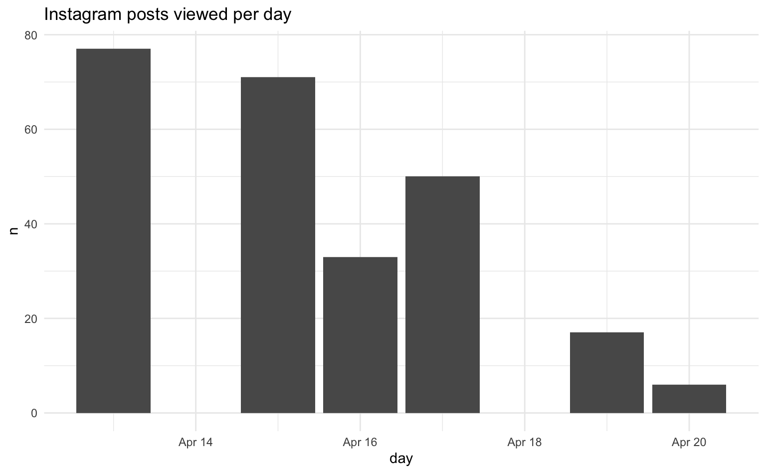
# Uhrzeit
insta_views |>
  count(hour) |>
  ggplot(aes(x = hour, y = n)) +
  geom_col() +
  labs(title = "Instagram posts viewed per hour of day")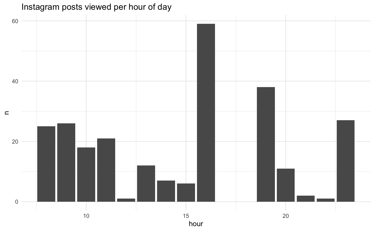
# Wochentage
insta_views |>
  count(weekday) |>
  ggplot(aes(x = weekday, y = n)) +
  geom_col() +
  labs(title = "Instagram posts viewed per day of the week")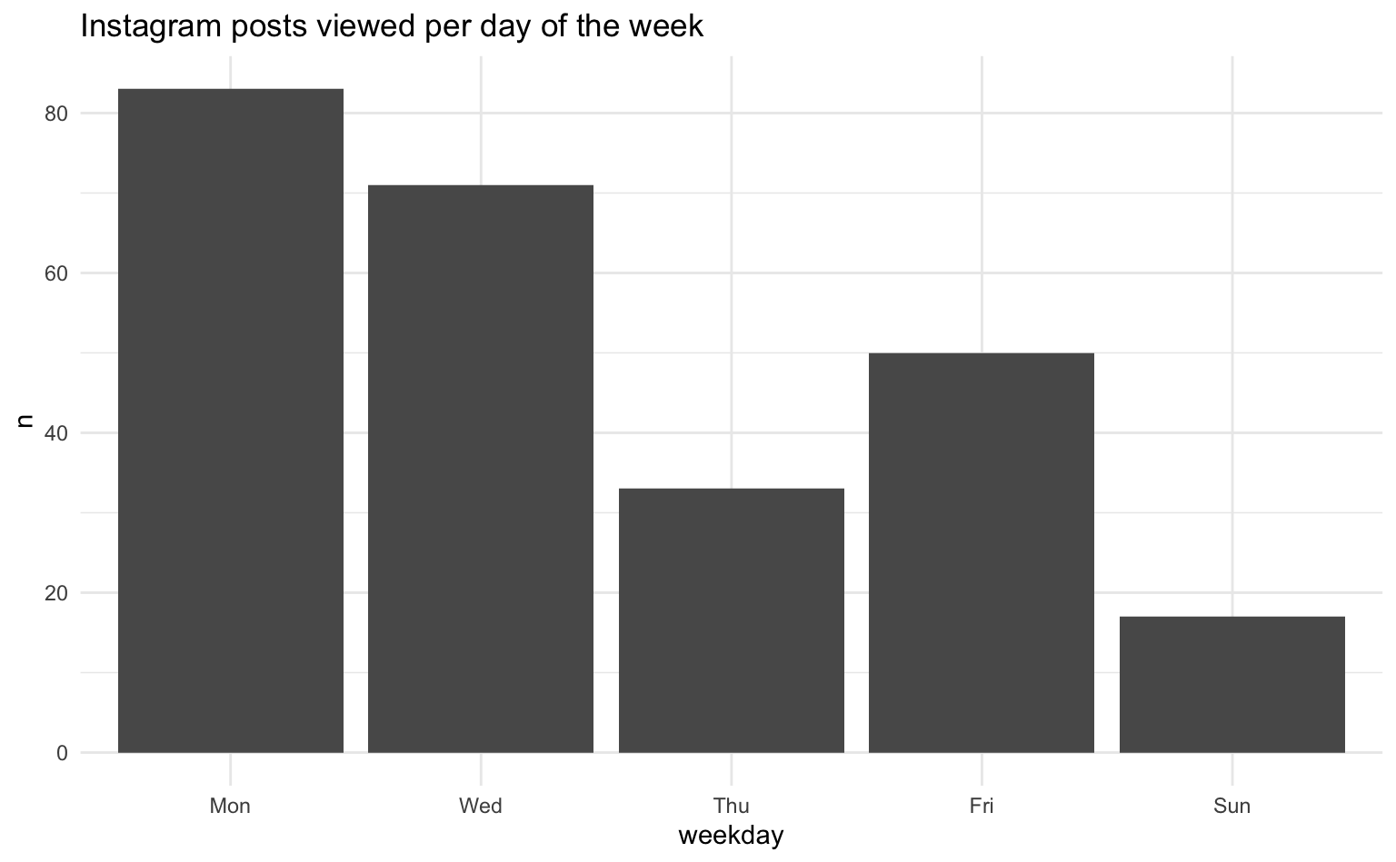
Wir können uns auch die Accounts anschauen, denen der Instagram-Account folgt.
Zunächst laden wir den Following-Verlauf aus einer JSON-Datei namens following.json sowie das Objekt relationships_following. Manche JSON-Dateien sind direkt eine Liste von Einträgen, andere haben eine weitere Schachtelung auf der obersten Ebene — das können wir mit names() prüfen. Wenn dort z.B. relationships_following steht, müssen wir eine Ebene tiefer gehen und relationships_following mit aufnehmen. Die Anzahl von Ebenen kann sich von Datei zu Datei unterscheiden. Die Daten werden wie oben umbenannt, ausgewählt und transformiert.
raw <- jsonlite::fromJSON("following.json")

names(raw)
[1] "relationships_following"insta_follow <- jsonlite::fromJSON("data/following.json")$relationships_following |>
unnest(string_list_data) |>
select(account = title, url = href, timestamp) |>
mutate(
timestamp = as.POSIXct(timestamp, origin = "1970-01-01"),
day = as.Date(timestamp),
hour = lubridate::hour(timestamp),
weekday = lubridate::wday(timestamp, label = TRUE, week_start = 1)
)Nun möchten wir die gefolgten Accounts zusammenfassen. Dazu erstellen wir ein Summenobjekt, mit dem Datum, der Anzahl Followings an diesem Tag sowie der kumulativen Summe.
insta_follow_counts <- insta_follow |>
  count(day) |>
  mutate(cumulative_n = cumsum(n))

insta_follow_counts
# A tibble: 3 × 3
day n cumulative_n
<date> <int> <int>
1 2026-04-10 15 15
2 2026-04-15 3 18
3 2026-04-16 2 20Mithilfe des Pakets ggplot2 können wir uns die Followings im Zeitverlauf in einem Liniendiagramm anschauen.
insta_follow_counts |>
  ggplot(aes(x = day, y = cumulative_n)) +
  geom_line(group = 1) +
  labs(title = "Instagram followings over time")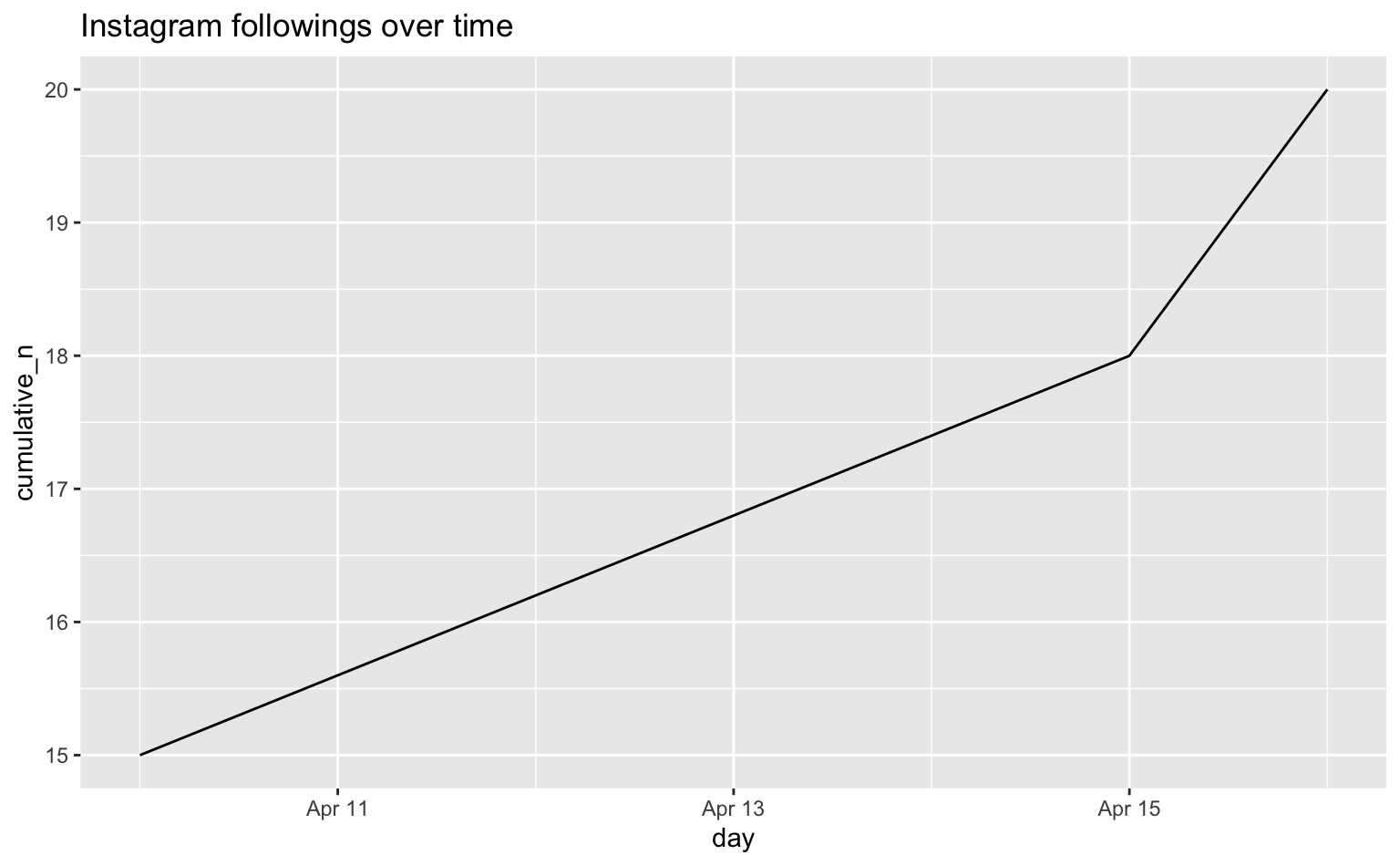
4.3 TikTok
Wir laden die TikTok-Nutzerdaten aus einer JSON-Datei namens user_data_tiktok.json. Die JSON-Datei enthält mehrere Felder mit interessanten Daten, was wir uns mit names() anschauen können. Hier sind die Variablen und Listen etwas anders geschachtelt als bei Instagram.
tiktok <- jsonlite::fromJSON("data/user_data_tiktok.json")
names(tiktok)
[1] "Comment" "Direct Message" "Income+ Wallet"
[4] "Likes and Favorites" "Location Review" "Post"
[7] "Profile And Settings" "TikTok Live" "TikTok Shop"
[10] "Your Activity" Hier analysieren wir den Verlauf der TikTok-Anmeldungen, um Muster in der Zugriffshäufigkeit über die Zeit hinweg zu erkennen. Wir extrahieren den Anmeldeverlauf aus den geladenen TikTok-Daten und wandeln ihn zur leichteren Bearbeitung und Analyse in eine Tibble um. Anschließend erstellen wir aus der Datumsspalte, die eine analysierbare Zeichenkette ist, neue zeitliche Variablen – Tag, Stunde und Wochentag. Dies ermöglicht es uns, die Anmeldehäufigkeit über verschiedene Zeitskalen hinweg zu analysieren.
tt_logins <- tiktok$`Your Activity`$`Login History`$LoginHistoryList |>
  as_tibble()

tt_logins
# A tibble: 12 × 6
Date IP DeviceModel DeviceSystem NetworkType Carrier
<chr> <chr> <chr> <chr> <chr> <chr>
1 2026-04-15 12:38:52 134.93.211.46 iPhone13,4 iOS 26.3.1 Wi-Fi ""
2 2026-04-15 22:00:05 77.25.2.63 iPhone13,4 iOS 26.3.1 Wi-Fi ""
3 2026-04-15 22:12:34 77.25.2.63 iPhone13,4 iOS 26.3.1 Wi-Fi ""
4 2026-04-15 22:15:33 77.25.2.63 iPhone13,4 iOS 26.3.1 Wi-Fi ""
5 2026-04-16 07:37:31 176.7.211.242 iPhone13,4 iOS 26.3.1 5g ""
# ℹ 7 more rowstt_logins <- tt_logins |>
mutate(
day = as.Date(Date),
hour = lubridate::hour(Date),
weekday = lubridate::wday(Date, label = TRUE, week_start = 1)
)
tt_logins# A tibble: 12 × 9
Date IP DeviceModel DeviceSystem NetworkType Carrier day hour
<chr> <chr> <chr> <chr> <chr> <chr> <date> <int>
1 2026-04-1… 134.… iPhone13,4 iOS 26.3.1 Wi-Fi "" 2026-04-15 12
2 2026-04-1… 77.2… iPhone13,4 iOS 26.3.1 Wi-Fi "" 2026-04-15 22
3 2026-04-1… 77.2… iPhone13,4 iOS 26.3.1 Wi-Fi "" 2026-04-15 22
4 2026-04-1… 77.2… iPhone13,4 iOS 26.3.1 Wi-Fi "" 2026-04-15 22
5 2026-04-1… 176.… iPhone13,4 iOS 26.3.1 5g "" 2026-04-16 7
# ℹ 7 more rows
# ℹ 1 more variable: weekday <ord>Anschließend können wir die Häufigkeit der TikTok-Anmeldungen visualisieren, indem wir die Anzahl der Anmeldungen pro Wochentag zählen und danach in einem Balkendiagramm darstellen.
tt_logins |>
  count(weekday) |>
  ggplot(aes(x = weekday, y = n)) +
  geom_col() +
  labs(title = "TikTok logins per day of the week")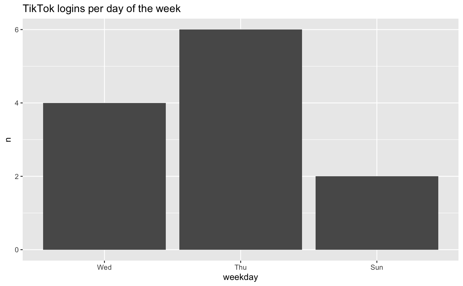
Im nächsten Schritt untersuchen wir den Verlauf der angesehenen TikTok-Videos, um Muster von genutzten Inhalten im Zeitverlauf zu verstehen. Die Vorgehensweise ist dieselbe wie oben, einschließlich der Umwandlung der Zeitstempel in mehrere Variablen - dieses Mal allerdings gebündelt.
tt_views <- tiktok$`Your Activity`$`Watch History`$VideoList |>
  as_tibble() |>
  mutate(
    day = as.Date(Date),
    hour = lubridate::hour(Date),
    weekday = lubridate::wday(Date, label = TRUE, week_start = 1)
  )

tt_views
# A tibble: 160 × 5
Date Link day hour weekday
<chr> <chr> <date> <int> <ord>
1 2026-04-15 12:39:05 https://www.tiktokv.com/share/vi… 2026-04-15 12 Wed
2 2026-04-15 12:39:14 https://www.tiktokv.com/share/vi… 2026-04-15 12 Wed
3 2026-04-15 12:39:15 https://www.tiktokv.com/share/vi… 2026-04-15 12 Wed
4 2026-04-15 12:41:50 https://www.tiktokv.com/share/vi… 2026-04-15 12 Wed
5 2026-04-15 12:41:51 https://www.tiktokv.com/share/vi… 2026-04-15 12 Wed
# ℹ 155 more rowsZu beachten ist, dass die Daten nur die URL des angesehenen Videos enthalten, jedoch keine zusätzlichen Metadaten. Diese Daten müssten wir in einem separaten Schritt erfassen und verknüpfen. Vorerst aggregieren wir die Daten zum Viewing-Verlauf, indem wir die Anzahl der an jedem Tag der Verlaufsdatei angesehenen Videos zählen und die Ergebnisse als Balkendiagramm darstellen.
tt_views |>
  count(day) |>
  ggplot(aes(x = day, y = n)) +
  geom_col() +
  labs(title = "TikTok videos watched per day")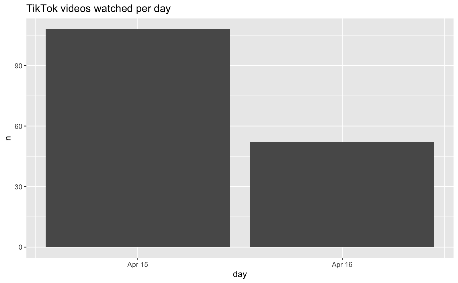
Schließlich untersuchen wir den Verlauf der Direktnachrichten auf TikTok, um Kommunikationsmuster zu verstehen, wobei wir uns auf die Häufigkeit von Nachrichten mit verschiedenen Nutzenden konzentrieren. Wir laden den Verlauf der Direktnachrichten aus den TikTok-Daten herunter. Da der Chat-Verlauf möglicherweise als Liste von „dataframes“ strukturiert ist, verwenden wir bind_rows(), um diese zu einem einzigen Tibble zusammenzufassen.
tt_dm <- tiktok$`Direct Message`$`Direct Message`$ChatHistory |>
  bind_rows() |>
  as_tibble()

tt_dm
# A tibble: 3 × 3
Date From Content
<chr> <chr> <chr>
1 2026-04-15 12:41:33 user4912600155075 Hier ist ein Test zurück
2 2026-04-15 12:40:51 alicia.ernst 🥳🥳🥳
3 2026-04-15 12:40:42 alicia.ernst Hi das ist ein Test Um die Kommunikationshäufigkeit mit verschiedenen NutzerInnen zu verstehen, zählen wir die Anzahl der von jedem Nutzer gesendeten Nachrichten (identifiziert durch die Variable „From“) und stellen die Ergebnisse in absteigender Häufigkeit dar.
tt_dm |>
  count(From, sort = TRUE)
# A tibble: 2 × 2
From n
<chr> <int>
1 alicia.ernst 2
2 user4912600155075 1Aufgabe
Analysieren Sie Ihren eigenen Takeout.
Wie viele Instagram vs. TikTok-Beiträge (falls beides vorhanden) schauen Sie durchschnittlich pro Tag an?
Welche Daten finden sich noch in den JSON-Dateien? Was könnte man mit ihnen analysieren?
Untersuchen Sie eine weitere Variable von Instagram und/oder TikTok (je nach vorhandener Takeout-Datei)